In this article, you’re going to learn how to use the Excel Functions Index and Match.
What Index Does
This function gives you the value of a cell in a range based on its row and column number.
What Match Does
This function finds the position of a value in a range. It tells you where the value is located, not the value itself.
Examples of Index Function
Remember that this function gives you the value of a cell in a range based on its row and column number.
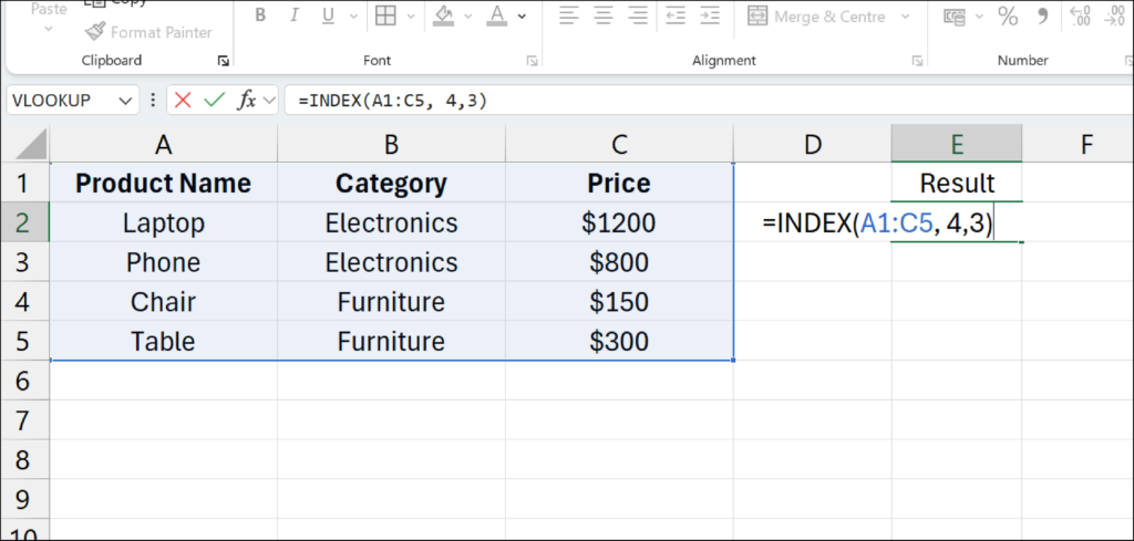
Below is the completed example of the Index function we’ll be writing out:

As you write out the INDEX function, there are parameters that need to be set. The Index function will look something like this, before it is written out:
=INDEX(array, row_num, [column_num])
Step 1: In any empty cell input =INDEX(
Step 2: The ‘array’ is the table you want the function to search through. Select the “array” (Table) then input comma.
Step 3: Set the ‘row_num’ to, in this case, 4. The function will look through the 4th row. Input comma.
Step 4: Set the ‘[column_num]’ to, in this case, 3. The function will look through the 3rd column. Input comma.
Step 5: End the function with a closed parenthesis (a closed bracket). The function should look like this: =INDEX(A1:C5, 4,3). Press ENTER
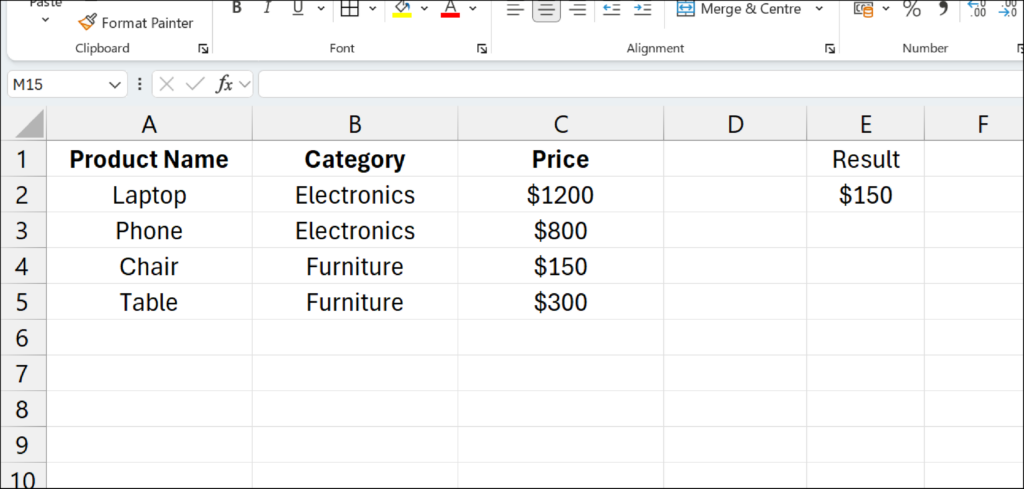
Result shown in cell E2:

The answer is $150. We directed the function to look through our array (our table) and within the 4th row and the 3rd column, then to return the data in that cell.
Try writing an Index function yourself. Try changing the row and column numbers so you get a different answer.
Remember that the Index Function gives you the value in a range based on its column and row number.
Examples of Match Function
Remember that this function finds the position of a value in a range. It tells you where the value is located, not the value itself.
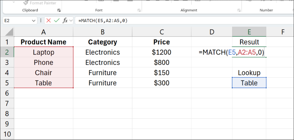
Below is the completed example of the Match function we’ll be writing out:

As you write out the MATCH function, there are parameters that need to be set. The Match function will look something like this, before it is written out:
=MATCH(lookup_value, lookup_array, [match_type])
Step 1: In any empty cell, input =MATCH(
Step 2: Set the ‘lookup_value’—the item you want the function to find a match for.. In this case it is cell E5, which has the word “Table” inside of it. You can also input data into this parameter like this: =MATCH(“Table”, rather than referencing a cell. In this scenario we are referencing a cell.
Step 3: For the ‘lookup_array,’ select the column you would like the function to look through.
Step 4: Set ‘[match_type]’ to 0 (zero), so you get an exact match for your answer.
Step 5: Press Enter.
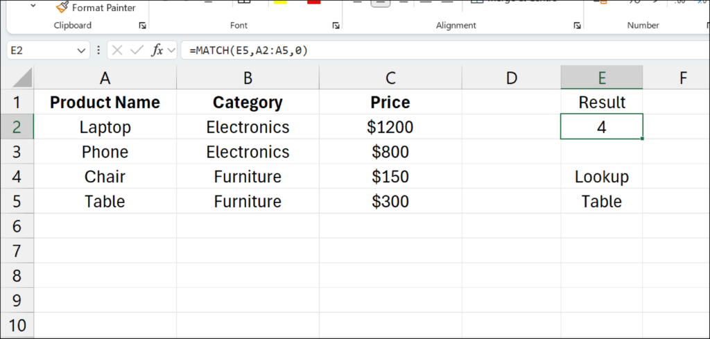
The result shown in cell E2:

In this case the answer is 4. This is because the word “Table” is located 4 cells from the top of the array (The column of data you selected for the ‘lookup_array’).