What is the DISC Function?
DISC is a financial function that allows you to calculate the discount rate of a bond.
DISC Formula & Parameters
The Excel function is written in the following manner:
=DISC(settlement, maturity, pr, redemption, [basis])
Parameters
- Settlement (required) – This is the date of purchase of the coupon. Also known as the settlement date, aka the date when the security is sold to the buyer.
- Maturity (required) – The date on which the security expires.
- Pr (required) – The price per $100 face value.
- Redemption (required) – The redemption value per $100 face value.
- Basis (optional) – The day count basis, possible values are:
| Basis | Day Count basis |
|---|---|
| 0 or blank | US(NASD) 30/360 |
| 1 | Actual/actual |
| 2 | Actual/360 |
| 3 | Actual/365 |
| 4 | European 30/360 |
Examples of the DISC Function
Example 1
Suppose we have the following data in our spreadsheet, this is how you apply the DISC function:
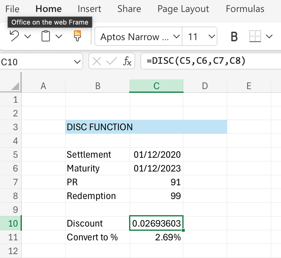
Note that we skipped the basis argument so the function took it as 0, which means it applies the US (NADS) 30/360 day count basis. If you need a different basis then refer to the parameters section above.
Important Points about the DISC Function
You could possibly get a #NUM! error if:
- Inputs for the arguments pr, redemption or basis are invalid values such as not being numbers
- Or if pr or redemption are less than or equal to 0
- Maturity date is before or on the settlement date (no-one buys an expired bond!)
- Settlement, maturity, and basis have been auto shortened to integers
#VALUE! error can be presented if:
- The given maturity date or settlement date is not a valid Excel date
- Any of the arguments are non-numeric values
Click here to download a copy of the DISC function worksheet.